Custom geometry: district-level NTL with custom boundaries
Source:vignettes/custom-geometry.Rmd
custom-geometry.Rmdlightson accepts any sf polygon layer. The
workflow below starts with the bundled LGD state boundaries, then swaps
in district-level GeoJSONs from bharatviz.
State-level workflow (bundled boundaries)
library(lightson)
library(sf)
#> Linking to GEOS 3.12.1, GDAL 3.8.4, PROJ 9.4.0; sf_use_s2() is TRUE

states <- get_india_admin("state")
nrow(states)
#> [1] 36
head(states[, c("state_name", "state_code")])
#> Simple feature collection with 6 features and 2 fields
#> Geometry type: GEOMETRY
#> Dimension:     XY
#> Bounding box:  xmin: 76.7052 ymin: 6.7528 xmax: 97.4129 ymax: 30.7941
#> Geodetic CRS:  WGS 84
#> # A tibble: 6 × 3
#>   state_name        state_code                                          geometry
#>   <chr>             <chr>                                         <GEOMETRY [°]>
#> 1 A & N Islands     35         GEOMETRYCOLLECTION (POLYGON ((92.4043 10.7844, 9…
#> 2 Andhra Pradesh    37         MULTIPOLYGON (((80.7879 15.7605, 80.79048 15.764…
#> 3 Arunachal Pradesh 12         POLYGON ((96.1765 29.3452, 96.1799 29.3075, 96.2…
#> 4 Assam             18         MULTIPOLYGON (((91.5352 25.8839, 91.5304 25.8713…
#> 5 Bihar             10         POLYGON ((84.1093 27.5208, 84.1242 27.5108, 84.1…
#> 6 Chandigarh        04         POLYGON ((76.7723 30.7941, 76.7828 30.7892, 76.7…
Download Bhuvan WMS rasters for a subset of years.
bhuvan_raster() derives the bounding box from the
geometry:
rasters <- bhuvan_raster(states, years = 2020:2022)
#> Downloading Bhuvan WMS: year 2020 ...
#> Downloading Bhuvan WMS: year 2021 ...
#> Downloading Bhuvan WMS: year 2022 ...
names(rasters)
#> [1] "2020" "2021" "2022"
rasters[["2022"]]
#> class       : SpatRaster
#> size        : 1024, 1024, 1  (nrow, ncol, nlyr)
#> resolution  : 0.0285501, 0.02962432  (x, y)
#> extent      : 68.1776, 97.4129, 6.7528, 37.0881  (xmin, xmax, ymin, ymax)
#> coord. ref. : lon/lat WGS 84 (EPSG:4326)
#> source(s)   : memory
#> varname     : file279f3c0f2837
#> name        : file279f3c0f2837_1
#> min value   :                 10
#> max value   :           245.9732
Bhuvan WMS returns RGB visualisation tiles, not physical radiance.
bhuvan_raster() converts to single-band luminance via
lum = 0.2126*R + 0.7152*G + 0.0722*B (ITU-R BT.709). Values
are comparable across years for trend analysis but are not in
nW/cm^2/sr.
panel <- extract_panel(rasters, states, id_col = "state_name")
#> Warning in st_cast.GEOMETRYCOLLECTION(X[[i]], ...): only first part of
#> geometrycollection is retained
head(panel)
#>         region_id year mean_radiance n_pixels
#> 1   A & N Islands 2020      72.73280        1
#> 37  A & N Islands 2021           NaN        0
#> 73  A & N Islands 2022      72.73280        1
#> 2  Andhra Pradesh 2020      89.00605     5425
#> 38 Andhra Pradesh 2021      89.06904     5619
#> 74 Andhra Pradesh 2022      85.62903     9063
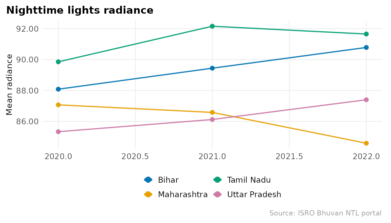
library(ggplot2)
sel <- c("Bihar", "Maharashtra", "Tamil Nadu", "Uttar Pradesh")
plot_ntl_trend(
  panel[panel$region_id %in% sel, ],
  region   = sel,
  caption  = "Source: ISRO Bhuvan NTL portal"
)
plot_ntl_map(
  rasters[["2022"]],
  polygons = states,
  title    = "India nighttime lights, 2022"
)
#> Warning: Raster pixels are placed at uneven horizontal intervals and will be shifted
#> ℹ Consider using `geom_tile()` instead.
#> Raster pixels are placed at uneven horizontal intervals and will be shifted
#> ℹ Consider using `geom_tile()` instead.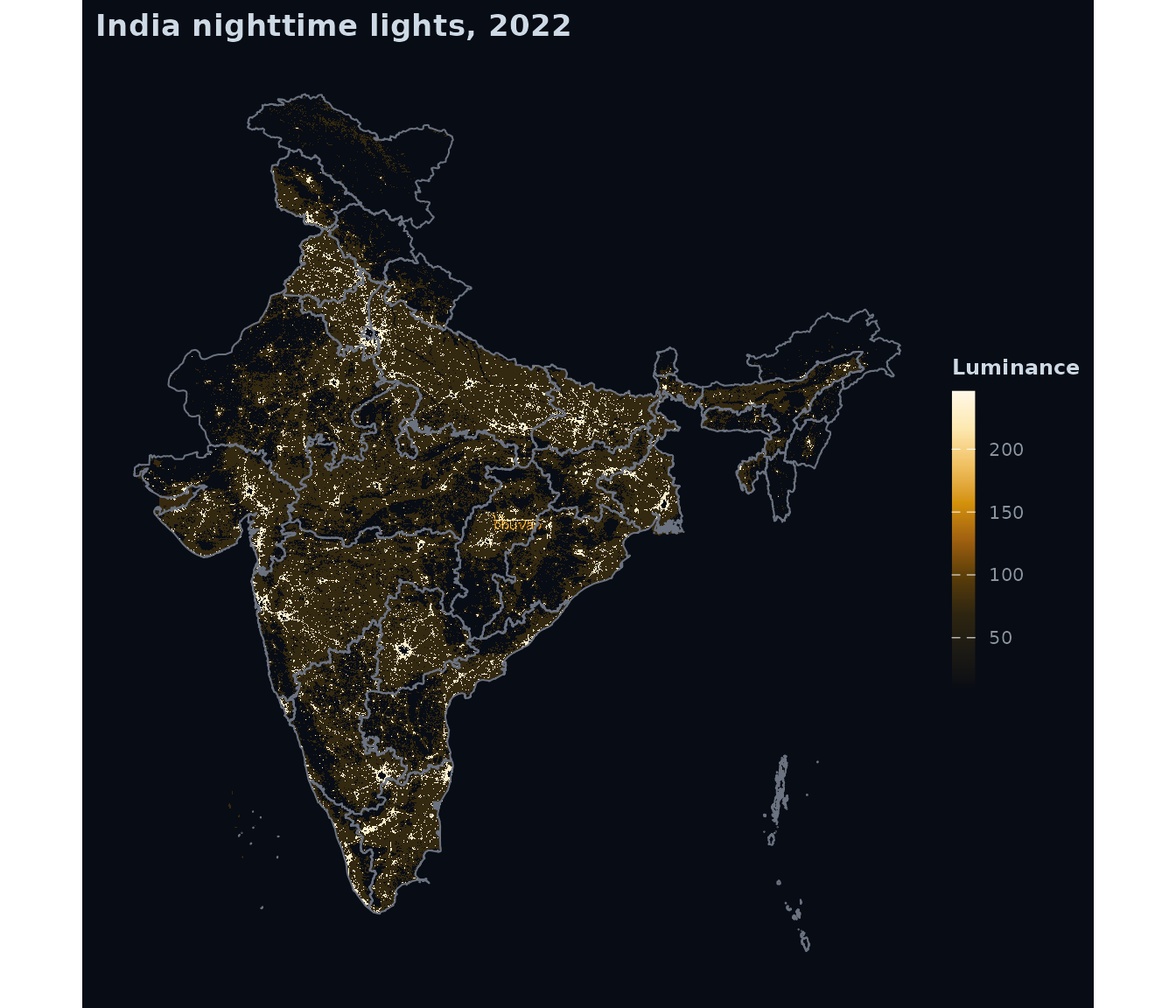
District-level workflow
BHARATVIZ <- "https://bharatviz.org"

districts <- tryCatch(
  sf::read_sf(file.path(BHARATVIZ, "India-bhuvan-districts.geojson")),
  error = function(e) NULL
)
#> Warning in CPL_read_ogr(dsn, layer, query, as.character(options), quiet, : GDAL
#> Error 4: Failed to read TopoJSON data
if (is.null(districts)) {
  message("bharatviz not reachable -- skipping district examples")
  knitr::opts_chunk$set(eval = FALSE)
}
#> bharatviz not reachable -- skipping district examples
nrow(districts)
#> NULL
rasters_dist <- bhuvan_raster(districts, years = 2018:2023)
names(rasters_dist)
panel_dist <- extract_panel(rasters_dist, districts, id_col = "district_name")
head(panel_dist)
plot_ntl_trend(panel_dist, region = c("Mumbai", "Delhi", "Chennai", "Bengaluru"))
plot_ntl_map(rasters_dist[["2022"]], polygons = districts)LGD boundaries
lgd <- sf::read_sf(file.path(BHARATVIZ, "India_LGD_districts.geojson"))
panel_lgd <- extract_panel(rasters_dist, lgd, id_col = "district_name")
head(panel_lgd)
Historical census boundaries
dist_2011 <- sf::read_sf(file.path(BHARATVIZ, "India-2011-districts.geojson"))
panel_2011 <- extract_panel(rasters_dist, dist_2011)
head(panel_2011)
extract_panel() picks the first character column as
region_id automatically, or pass id_col
explicitly.
VIIRS path
To use NASA VIIRS rasters, supply an Earthdata token:
token <- earthdata_token()
rasters_viirs <- ntl_download("viirs", region = districts, years = 2018:2023, token = token)
if (length(rasters_viirs) > 0) {
  panel_viirs <- extract_panel(rasters_viirs, districts, id_col = "district_name")
  head(panel_viirs)
}